
 Share This Page
| Home | | Mathematics | | * Applied Mathematics | | * Storage Tank Modeling | |  |  |  Share This Page Share This Page |
Copyright © 2009, Paul Lutus — Message Page
(double-click any word to see its definition)

Full VolumeThis page provides mathematical methods and Java code to compute full and partial volumes for first- and second-order trapezoidal storage tanks (first-order tanks have a trapezoidal cross-section in one dimension, second-order in two dimensions). Trapezoidal tanks are mathematically simpler than the elliptical and tilted tanks that are the primary focus of this department of arachnoid.com, but they are sufficiently complex, and I have received enough inquiries about them, that I think they deserve their own page.
This page also provides some useful general mathematical methods and is structured as a tutorial, so it may be worth reading even if the reader doesn't have an immediate need for its results.
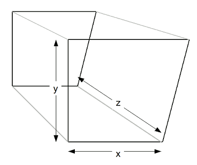
The full volume for a first-order trapezoidal tank is quite easy to compute, but first let's adopt a variable naming convention to be used through this entire exercise. As shown in Figure 1, let:
- x = horizontal dimension (left-right)
- y = vertical dimension (up-down)
- z = depth (in-out)
Figure 1 shows that the x dimension of the tank is different at the bottom than at the top, so we'll use the name xb to refer to the x dimension's bottom width and xt to refer to the x dimension's top width. Computing the full volume for this tank type is then very easy:
(1)
That's fine for a full volume result, but it would be useful to obtain intermediate volume results — a volume for each content height in the tank as measured by a level sensor, for example. It should be obvious that each intermediate height of a trapezoidal tank is computed the same way that the full tank is, but it's not obvious what the intermediate x widths should be for each height in the y dimension — that will be our next task.

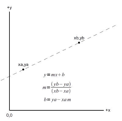
Line to Surface to VolumeThis very useful method requires two defined data pairs (xa,ya and xb,yb) as shown in Figure 2. Given these two defined points, we can compute intermediate y values for provided x arguments. The desired intermediate y values are computed using a method called "linear interpolation," a way to translate one numerical range to another ("interpolation" means computing intermediate values between defined points). Here is the classical way to express this idea:
(2)
If given an x argument, equation (2) creates a y result that has been shifted and scaled to agree with any desired linear transformation. In this context, "linear" means a graphical representation will produce a straight line passing through two defined data points as in Figure 2.
Two new variables appear in equation (2): m and b. Here is how to compute m:
(3)
Having gotten a value for m, here is how to compute b:
(4)
Equations (2) through (4) show the classical form of linear interpolation that predates the computer era, a time when these results were likely to be acquired through hand calculation. In that time it was desirable to break the calculation into as many individual steps as possible to avoid errors and make the process more manageable. Now that we have computers to help us, we can use a combined equation that eliminates the need to separately compute m and b:
(5)
For equation (5), instead of computing m and b, we directly use the two data pairs (xa,ya and xb,yb) shown in Figure 2. For our tank problem we have the required data pairs — they represent the bottom and top y values for the interval for which a volume result is needed, and two x widths corresponding to the y values.
From a technical standpoint, equation (5) first "normalizes" the range of x values — that is, it makes them fall between zero and one. The equation then scales this normalized result using the provided y range defined by yb-ya, and finally the result is shifted by adding the ya value. This process has the effect of translating the x numerical range to the domain defined by the y values, so that when x = xa, y = ya and when x = xb, y = yb, and more important, any intermediate x values produce corresponding intermediate y values (the dashed line in Figure 2).At this stage the astute reader will notice that the linear interpolation equations use x as an argument and y as a result, while the tank problem assumes the opposite (x and y are reversed). I ask the reader to mentally switch the meaning of x and y when considering a tank-specific calculation, or (depending on personal taste) mentally rotate the tank's coordinate system 90 degrees to accommodate the fact that it is the x dimension's width that needs to be computed for any provided y argument.
I want to emphasize to young programmers how useful equation (5) is — I find myself applying it again and again in my programs, to solve various problems in a clearly defined way. For example, most of my graphics programs auto-scale their displays when the user resizes the application frame — this is done using a version of equation (5). Another common application converts from one defined numerical range to another, for example from Celsius to Fahrenheit:
Define:Result:
- xa = 0
- xb = 100
- ya = 32
- yb = 212
0 32 10 50 20 68 30 86 40 104 50 122 60 140 70 158 80 176 90 194 100 212 Readers may wonder whether this method is more complex than it needs to be — can't we just multiply the x values by a single constant term to get the desired y results? Well, no, that would mean that when x = 0, y = 0 and this would represent a serious practical limitation. Equation (5) is only as complex as it needs to be, and no more.
Height for VolumeAbove we created a way to compute a width, a one-dimensional line, in the x dimension for a given y height in our tank. In this step we will compute a two-dimensional surface area for a given y argument, then we will create a volume result.
The mathematical reader will see that we're now moving into Calculus — the transition from a one-dimensional line to a two-dimensional area, then to a a three-dimensional volume, requires the Calculus idea of integration. (For those interested in learning more about Calculus, I recommend my Calculus Tutorial) The first-order trapezoidal tank's integrals are very simple, and I mention this connection with Calculus only to clarify the underpinnings of the method. (Later on, when we evaluate second-order trapezoids, the integrals become more complex).
To move from a line to a surface area we have to add the tank's third dimension z, which has been ignored until now:
(6)
Because this is a first-order trapezoid, variable z is a constant (meaning the z width is the same at the bottom and top of the tank), consequently this calculation is relatively simple. In equation (6) the result a represents the two-dimensional surface area for any provided y height in the tank.
In the next step, we integrate equation (6) on the interval between yb (the tank bottom) and y (the desired content height), like this:
(7)
Equation (7) provides the desired result volume, expressed in cubic units in which x, y, and z are provided, for a given y height.
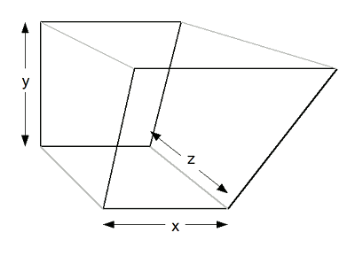
Figure 3: Equivalent VolumesSome correspondents have asked whether this tank computation is made more complicated by the fact that (unlike Figure 1) both sides of the tank are sometimes tilted (in a single dimension) — doesn't this make the computation more complex? Well, no, and here's why. Imagine a stack of rectangular blocks with different widths. It doesn't matter whether the blocks are stacked so that one side of the stack is vertical, or so that neither side is vertical — the total volume of the blocks doesn't change. Now imagine a nearly infinite stack of nearly infinitely thin blocks, and this example becomes the volume integral for our tank. Remember this when measuring your tank — the width of the tank is all that matters, not the angles of the sides.
Equation (7) produces a volume v for any given content height y. Can it be reordered to produce a height for a provided volume, the reciprocal case? Yes — here is that form:
(8)
Because these equations are becoming rather complex, I should say that a general-purpose Java program is provided later in this article that produces a large variety of result types, including tables of volumes for heights and the reverse, for both first-order and second-order trapezoidal tanks.

Java ProgramThis section deals with the case of a tank whose width changes in both the x and z dimensions, that is, a second-order trapezoidal solid (see Figure 4). For this case we need to provide two new values (zb and zt) for the additional dimension, and two simultaneous interpolations are carried out in the following equations (for the x and z dimensions), both with respect to y. It almost goes without saying that the additional dimension greatly increases the complexity of the associated equations, to the degree that it becomes very difficult to use them in a spreadsheet — one is almost required to create a computer program to manage the computations. (See below for a general-purpose Java program that manages all the described forms.)
Here is the surface area equation for the second-order trapezoid:
(9)
And here is the corresponding volume integral on the interval yb to y (note the scroll bar at the bottom of the graphic):
(10)
Unfortunately, the second-order trapezoidal integral of equation (10) has some properties that prevent the creation of the popular and much-requested reciprocal (height for volume) form. The reason is a bit technical but it has to do with information irretrievably lost during the volume integration. But don't despair — the Java program described below gets around this problem and provides heights for volumes.
At this point the reader may wonder how one can check the results for an equation as complex as equation (10) — how can we be sure it provides accurate results for a second-order trapezoidal solid? Well, there are some canonical geometric forms for which there are simple expressions, such as a pyramid, and dimensions for a pyramid can be submitted to equation (10). A pyramid's volume is defined as:
(11)
Using the Java program below, we discover that the simple pyramid volume is correctly predicted. There are other more subtle accuracy tests, but the pyramid result is an easily understood accuracy confirmation.
Volume ConversionsBecause of the complexity of the second-order case, and because I wanted a single solution for all the described tank types, I have written a Java program that produces all combinations of:
- First-order and second-order trapezoidal tanks.
- Volume for height and height for volume.
- Individual results and data table generation.
Here are download options:
- Click here to see a pretty-printed listing of the Java program.
- Click here to download the Java source code in plaintext form.
- Click here to download the executable Java class file.
To use the Java class file:
- Download the Java class file linked above.
- Place the class file in any convenient directory.
- Open a shell session (Windows: a "command prompt") and move to the directory where the class file is located.
- Execute the program with no arguments to see its options:
java RectTankVolume
- Result:
Usage: -v(olume for height) or -h(eight for volume), x bottom width, x top width, z bottom width, z top width, y bottom value, y top value, single argument for one result or start, end, step size for table of results (all on one line, delimited by spaces)- Here is an example that creates a table of volumes for sensor heights:
java RectTankVolume -v 5 10 7 12 0 10 0 10 1Here is a detailed description of the above entry:
- "-v" means "provide volumes for heights". The alternative is "-h", meaning heights for volumes. One or the other of these values must be present.
- "5 10" describe the bottom and top widths of the tank's x dimension (xb and xt)
- "7 12" describe the bottom and top widths of the tank's z dimension (zb and zt). For a first-order tank (with parallel z sides), make both these numbers the same.
- "0 10" describe the y values corresponding to the x and z values. Normally this number pair specifies the bottom and top of the y tank measurement range (yb and yt).
- "0 10" describe the generated table starting and ending values. These numbers don't have to agree with yb and yt although they usually do.
- "1" describes the table step size, the interval between successive values. This value can be less than one, example "0.1" for steps of 1/10 measurement unit.
Here is the result table for the above example:
          Height,          Volume
        0.000000,        0.000000
        1.000000,       38.083333
        2.000000,       82.666667
        3.000000,      134.250000
        4.000000,      193.333333
        5.000000,      260.416667
        6.000000,      336.000000
        7.000000,      420.583333
        8.000000,      514.666667
        9.000000,      618.750000
       10.000000,      733.333333
Remember that the results are provided in the entry units cubed. If the tank dimensions have been provided in inches, the result is expressed in cubic inches. To convert cubic inches to gallons, divide by 231, and see below for a table of common conversions.Sanity Checks
- Cube Test:
java RectTankVolume -v 10 10 10 10 0 10 10- Result:
Height, Volume 10.000000, 1000.000000- Pyramid Test:
java RectTankVolume -v 10 0 10 0 10 0 10- Result:
          Height,          Volume
       10.000000,      333.333333
NotesHere is a table of common volume unit conversions. The left column shows input units and the top row shows output units. The table's data cells contain the appropriate conversion factor to convert from the left column units to the top row units.
Liter Gallon Meter3 1000 264.17205 Centimeter3 1/1000 1/3705.4 Millimeter3 1/1000000 1/3785411.8 Foot3 28.316847 7.4805195 Inch3 1/61.023744 1/231
DisclaimerThis Web page and the associated Java program are © Copyright 2009, P. Lutus. The Java program is released under the GPL.
Much of the preliminary mathematical work was performed using Mathematica, and some equations were exported from Mathematica, converted using a Mathematica -> OpenOffice Math equation editor translation algorithm written in Ruby, then rendered in, and exported from, the OpenOffice Math equation editor.
For some reason, over time it has become, not easier, but much harder, to write and render equations in a form suitable for display in a Web page. Many projects have been started to make mathematical equation rendering an integral and generic part of Web pages, but to date all of these projects have failed, some spectacularly.
By far the most difficult part of managing equations is that no two mathematical programs are willing to talk to each other — Mathematica, Maxima, Maple and other math programs use one export syntax (all different and mutually incompatible), each available equation editor uses a different syntax, and TeX uses yet another. Not one of these programs has a shared convention for describing and rendering equations. As a result, I spend a lot of time writing translation algorithms between my current favored mathematical work environment and another program more suitable for rendering the equations as graphic images.
I apologize for the strict legalese below, but this program's calculations may be used to design and maintain fuel tanks and the possibilities for litigation have not escaped my attention. Sorry. Disclaimer of WarrantyThe computations provided by this page and Java program are provided on an "as-is" basis, without warranty of any kind, including without limitation the warranties of merchantability, fitness for a particular purpose and non-infringement. The entire risk as to the quality and performance of the computations is borne by you. Should the results prove to be in error, you assume the entire cost of any required service and repair, and any consequential damage.Limitation of LiabilityAs customary in the computer business, you are solely responsible for any loss of profit or any other commercial damage, including but not limited to special, incidental, consequential or other damages. This disclaimer specifically disclaims all other warranties, expressed or implied, including but not limited to the implied warranties of merchantability and fitness for a particular purpose, related to defects in the computed results or the documentation.
| Home | | Mathematics | | * Applied Mathematics | | * Storage Tank Modeling | |  |  |  Share This Page Share This Page |