Share This Page
| Home | | Mathematics | | * Applied Mathematics | | * Storage Tank Modeling | | | Share This Page |
An in-depth look at storage tank volume measurement
Copyright © 2011, Paul Lutus — Message Page
Since I posted my volume computation engine TankCalc online a few years ago, I've received many inquiries about apparent errors, tank shapes that TankCalc can't handle, and general questions about the mathematics of volume computation. I hope to cover most such inquiries here.
Unlike TankCalc, this article discusses solutions that require user participation. In some cases it relies on TankCalc for preliminary results and then expands on them, in others it requires the user to apply provided equations or methods. My goal is to make my readers more self-sufficient in this kind of computation, and to go beyond what TankCalc (or any single program) can do.
A common error people make using TankCalc is to measure the outside dimensions of a tank and compute a volume on that basis. But the goal is to measure the tank's internal volume, using the outside dimensions. For that, we need to take the tank's wall thickness (wt) into account.
Once we know the tank's wall thickness, we can take external measurements, correct them for wall thickness, and apply them to TankCalc with a reasonable expectation that the volume results will be accurate. Like this:
- Acquire a wall thickness value for your tank. Call this value wt.
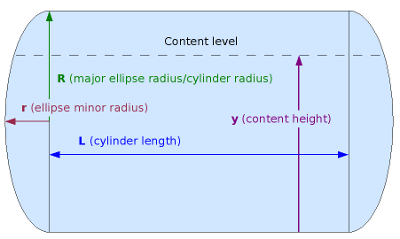
- Measure your tank externally to acquire the three values required by TankCalc (see Figure 1):
- L = tank cylindrical section length.
- R = radius of the cylindrical part (ellipse major radius).
- r = radius of the end cap (ellipse minor radius).
- Use the wall thickness to acquire corrected measurements (L',r',r'):
- L' = L unless the tank has flat end caps that don't extend beyond the end of the tank, in which case L' = L - 2wt.
- R' = R - wt
- r' = r - wt
- Use the corrected measurement values (L',R',r') in TankCalc to compute your tank's internal volume.
Also, notice that TankCalc can use a tank wall thickness to compute your tank's empty and full weight. Go to the "Tune" tab and notice the section titled "Surface Area, Mass". Enter the wall thickness and a density for the tank's material. A table of common material densities can be found in the help file and online as well.
Update: users may find it easier to analyze this tank type with the new TankProfiler program.
This is possibly the most common inquiry about TankCalc. To compute a volume table for a horizontally-mounted oval-cross-section tank, perform these steps:
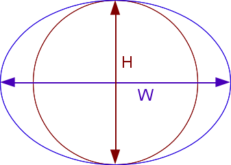
- Measure the tank's height (H) and width (W) in any convenient units.
- Use TankCalc to compute a table of results using only the height (H) measurement (divided by 2, then applied as TankCalc's R value), just as though the tank were the red cylinder shown in Figure 2. (This approach has the advantage that it correctly takes sensor measurement heights into account.)
- Export the table and paste it into a spreadsheet:
- You need to download TankCalc and run it locally for this procedure — download here (TankCalc is free).
- As explained above, create a table of values for a cylindrical tank that has your tank's height (H).
- At the "Compute" tab, press the "CSV" button to produce a comma-separated-values result table.
- Press the "Copy" button to copy the result table onto the system clipboard.
- Open a spreadsheet program and select menu item "Edit ... Paste".
- A dialog will open asking for some information about the pasted data. Choose a comma as the data delimiter. Click "OK".
- The TankCalc result table will appear in the spreadsheet.
- Now compute a width-to-height ratio for your tank:
- The width-to-height ratio is equal to an oval tank's width divided by its height.
- Example: if your tank has a width of 48" and a height of 36", the desired ratio is 48/36 = 1.3333...
- Return to the spreadsheet and locate the first volume result. Let's say for this example the cell address is B5.
- Move one spreadsheet cell to the right, and enter "= B5 * 1.33333".
- Copy this cell entry down the column for as many cells as there are volume results, so each volume result has the ratio number applied to it.
- This new column contains the correct volumes for your oval tank.
Some correspondents have asked why I don't just put this special case into TankCalc. My reply is that there are too many such variations to realistically include in a program that shouldn't become too complex for an untrained person to use.
Update: I've been getting a lot of inquiries about oval cross-section tanks, so I have written a Python script that manages this tank type. The script processes horizontally mounted, flat-ended cylindrical and oval cross-section tanks and produces two kinds of tables: sensor height to volume, and volume to sensor height. The user simply enters tank height, width, length, desired table step size, all in consistent units (i.e. inches, centimeters, etc.), and an optional volume conversion factor explained below. For each table type, the program emits a comma-separated data table ready to be pasted into a spreadsheet program for more processing or printing. Click here to see and download the script.
The script's default output units are the input units cubed, i.e. cubic inches for inches, cubic centimeters for centimeters, etc.. To convert to other volume units, simply add a conversion factor to the end of the argument list as explained in the program's help display (automatically shown if no arguments are entered).
Here is the program's help display:
The above is the simplest imaginable way to compute values for an oval tank, but it has a number of limitations. For a more comprehensive, flexible method, see TankProfiler.Usage: [-i(nverse mode)] (tank height) (tank width) (tank length) (table step size) [(conversion factor)] Conversion factors: cm³ -> liters: 1000, in³ -> gallons: 231
This refers to tanks that are essentially rectangular in cross-section, but that have one or more sloped sides. This brief section is only meant to link to my articles on this topic — it turns out I have written two articles about this kind of tank, each of which provides multiple resources for computing this tank type:
- Trapezoidal Storage Tanks (using Sage)
- Trapezoidal Storage Tanks (using Java)
I originally created these equations to be able to accurately mark plastic buckets at intermediate volume points. In the course of maintaining my boat I use buckets to hold measured quantities of lubricating oil prior to being pumped into my engine and transmission. Because I need to measure accurate amounts, I use these equations to mark my buckets at intermediate volume levels.
Since that initial task I've received a number of inquiries from TankCalc users, asking for volume solutions for this exact container shape. I realized I had already solved this case, so ... here it is.
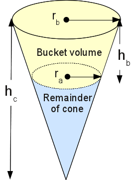
First, a bucket's volume is a section of a cone (technically a conical frustum), a well-defined geometric solid, so an obvious approach is to compute the volume of a hypothetical cone that includes the same widths as the top and bottom of the bucket, then subtract the remainder of the cone from the region of interest (see Figure 3, yellow).
Full Bucket Volume
The only variable not obtained by measurement, that must be computed, is hc, the height of the hypoethetical cone that the bucket is part of. Here is an equation for hc in terms of measured values:
Refer to Figure 3. Three of the required variables are defined by direct measurement:
- rb, the bucket's top rim radius and the base radius of the cone.
- ra, the bucket's bottom radius.
- hb, the bucket height.
(1) $\displaystyle h_c = \frac{h_{b}\ r_b}{r_b-r_a}$With equation (1) we can write a preliminary equation for the bucket volume bv:
(2) $\displaystyle bv = \frac{1}{3} \pi \, {\left( r_b^2 h_c - r_a^2 (h_c-h_b) \right)}$Because hc is defined by equation (1), equation (2) can be expanded to:
(3) $\displaystyle bv = -\frac{\pi h_{b} r_{b}^{3}}{3 \, {\left(r_{a} - r_{b}\right)}} + \frac{1}{3} \, {\left(\frac{h_{b} r_{b}}{r_{a} - r_{b}} + h_{b}\right)} \pi r_{a}^{2} $By combining terms and simplifying, equation (3) becomes:(4) $\displaystyle bv = \frac{1}{3} \, \pi \, h_b \, \left( r_a^2 + r_a r_b + r_b^2 \right)$Equation (4) provides a full volume for a bucket with the specified measurements. But it would be more useful to have an equation able to provide a partial volume for a given y height argument in the range 0 <= y <= h.
Partial Bucket Volume
First, for a conical frustum with radii ra and rb, and height h, let's write an equation that provides a circle area a for a provided argument y, 0 <= y <= h:
(5) $\displaystyle a = {\left(\frac{{\left(r_{a} - r_{b}\right)} y}{h} - r_{a}\right)}^{2} \pi$Now let's integrate equation (5) on the interval {0,y} to acquire a volume v:(6) $\displaystyle v = \int_0^y \, {\left(\frac{{\left(r_{a} - r_{b}\right)} z}{h} - r_{a}\right)}^{2} \pi \, dz = \frac{{\left(3 \, h^{2} r_{a}^{2} y + {\left(r_{a}^{2} - 2 \, r_{a} r_{b} + r_{b}^{2}\right)} y^{3} - 3 \, {\left(h r_{a}^{2} - h r_{a} r_{b}\right)} y^{2}\right)} \pi}{3 \, h^{2}} $Equation (6), created using Sage, provides a partial conical frustum volume v for a given height y. In a perfect world, an inverse equation would exist that would provide a height y for a partial volume v. Is there one in this case? Sage says yes:
(7) $\displaystyle y = \frac{h r_{a}}{r_{a} - r_{b}} - \frac{\left(\frac{{\left(\pi h r_{a}^{3} - 3 \, {\left(r_{a} - r_{b}\right)} v\right)} h^{2}}{\pi}\right)^{\frac{1}{3}}}{r_{a} - r_{b}}$Equations (6) and (7) are rather complex — maybe it would be a good idea to produce some test results. Let's say we have a conical frustum with this description:
- ra = 5
- rb = 10
- h = 10
Using Sage, we create a table of results — a series of y height arguments, a result volume v for each y from equation (6), and a result y for each volume v from equation (7). Here are the results:
y argument Equation(6): volume for y Equation(7): y for volume 1.0000 86.6556 1.0000 2.0000 190.5900 2.0000 3.0000 313.3739 3.0000 4.0000 456.5781 4.0000 5.0000 621.7735 5.0000 6.0000 810.5309 6.0000 7.0000 1024.4210 7.0000 8.0000 1265.0146 8.0000 9.0000 1533.8826 9.0000 10.0000 1832.5957 10.0000 It seems that, in a manner of speaking, equations (6) and (7) agree with each other. Click here for a simple Python script that calculates bucket profiles using the equations from this section. For a more general solution with more features, try TankProfiler.
This section describes methods for obtaining closed-form equations for certain tank types amenable to this approach. A later section discusses the more general (and less elegant) numerical computation method.
Computing volumes uses some ideas from Calculus, a field of mathematics that deals with movement and change. I'll be presenting just enough Calculus ideas to explain how one computes volumes, but those readers who would like a more complete Calculus exposition can click here.
Ideally, after analyzing a storage tank, we should be able to write a closed-form expression that describes its volume for any given measurement height. For this example, let's use the simplest nontrivial tank form — a cylindrical tank with flat ends, lying level on the ground. We want an equation that will provide partial volumes for any measured content height. After some thought, we decide to proceed this way:
- We have a measurement that tells us the height of the tank's contents, a one-dimensional value.
- We realize we can write an equation that provides a width within the tank for any height, and this is also a one-dimensional value.
- We can take the result of step (2) above and use Calculus methods to create an equation that represents the area of a slice of the tank's contents at any measured content height, a two-dimensional value.
- We can take the result from step (3) above and multiply by the tank's length, thus obtaining a partial tank volume, a three-dimensional result.
- By progressing from one dimension to three, we use Calculus ideas to move from a scalar measurement of tank content height to a volume.
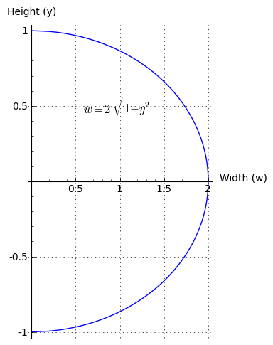
Figure 3: Width EquationStarting with step (2) above, let's think about an equation that will provide a content width w for any vertical location y in a normalized cylindrical tank (i.e. a tank with a radius of 1). (When writing equations, it's a good idea to write them in normalized form — such an equation represents the most general form and is easily scaled to represent an object in the real world.)
We realize the tank has zero width at the very bottom and top, and maximum width at the middle. After some geometric thinking, we come up with this candidate equation:
(8) $\displaystyle w = 2\ \sqrt{1-y^2}$
Where:
- y = normalized position within the tank, -1 ≤ y ≤ 1
- w = tank width (diameter) at y
A graph of our equation appears in Figure 3, and it correctly maps y values between -1 (bottom) and 1 (top), to a curve representing the width of our normalized tank.
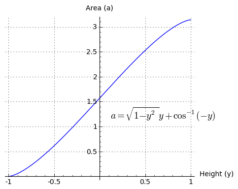
Next, we want to integrate equation (8), to produce a two-dimensional surface representing the area between the bottom of the tank and any given y value. This is the first step toward creating a three-dimensional volume.
Here is the integral of equation (8), which produces an area a for a unit circle section partitioned by argument y (-1 ≤ y ≤ 1):
(9) $\displaystyle a=\sqrt{1-y^2}y+\cos^{-1}(-y)$
Where:
- y = normalized vertical position within the tank, -1 ≤ y ≤ 1.
- a = area of the region between the bottom of the tank and a given y value.
Figure 4: Area EquationIn the final step, we use equation (9) to compute a tank volume for a real-world tank, one with radius r and length l, using these steps:
- Measure the tank's content height. Call this measured height h.
- Create a normalized height for use with equation (9): $ y = \frac{h}{r}-1$.
- Apply the normalized y value (with the range -1 ≤ y ≤ 1) to equation (9) to acquire a normalized area result a, which can assume values between 0 and $\pi$.
- Compute the tank's partial content volume v by multiplying the above area result by the tank's radius r squared, times length l:
$\displaystyle v = r^2 l \sqrt{1-y^2}y+\cos^{-1}(-y)$.- The volume result has the cubic form of the original measurement units.
There are many tank types, and tank orientations, that cannot be analyzed using closed-form equations. For these, numerical methods are required (and TankCalc relies almost completely on numerical results).
It's important to understand that numerical results are always approximate. One can improve the accuracy of a numerical result, but this usually involves increasing the amount of time required to arrive at a result.
This section involves algorithms and some computer programming, and I have chosen the computer language Python for the examples. Python is available for most platforms and is very easy to use.
Numerical integration is easy to explain — one produces an approximate integral by summing many individual results. One can improve the accuracy of the result by increasing the number of samples, but this increases runtime.
In this example we will compare an approximate numerical result with a known closed-form result, using the equations from the prior section. We will adjust the number of samples to see how this improves the accuracy of the result. The Python source for this example is here.
Here is a comparison for 100 samples:
y Closed-form Numerical Error % 0.2 0.163501 0.164649 +0.702320% 0.4 0.447295 0.450348 +0.682607% 0.6 0.792673 0.797902 +0.659602% 0.8 1.173479 1.180899 +0.632301% 1.0 1.570796 1.580209 +0.599199% 1.2 1.968113 1.979093 +0.557895% 1.4 2.348919 2.360763 +0.504205% 1.6 2.694297 2.705876 +0.429744% 1.8 2.978092 2.987400 +0.312577% 2.0 3.141593 3.138269 -0.105811% Here is a comparison for 1,000 samples:
y Closed-form Numerical Error % 0.2 0.163501 0.163619 +0.072382% 0.4 0.447295 0.447611 +0.070494% 0.6 0.792673 0.793215 +0.068287% 0.8 1.173479 1.174250 +0.065664% 1.0 1.570796 1.571778 +0.062478% 1.2 1.968113 1.969265 +0.058496% 1.4 2.348919 2.350171 +0.053309% 1.6 2.694297 2.695539 +0.046099% 1.8 2.978092 2.979126 +0.034733% 2.0 3.141593 3.141487 -0.003348% Finally, here is a comparison for 10,000 samples:
y Closed-form Numerical Error % 0.2 0.163501 0.163513 +0.007307% 0.4 0.447295 0.447327 +0.007121% 0.6 0.792673 0.792728 +0.006903% 0.8 1.173479 1.173557 +0.006644% 1.0 1.570796 1.570896 +0.006329% 1.2 1.968113 1.968230 +0.005935% 1.4 2.348919 2.349047 +0.005421% 1.6 2.694297 2.694424 +0.004706% 1.8 2.978092 2.978198 +0.003579% 2.0 3.141593 3.141589 -0.000106% From these examples, it's easy to see that accuracy gradually improves as the sample size goes up, but it's important to say that each improvement in accuracy of one decimal place requires a tenfold increase in runtime. There are some specialized methods to reduce this burden, but in general it's a consistent rule in numerical integration.
Here is the numerical integration function from the Python example code:
def num_int(f,ni,a,b):
  if(a == b): return 0
  nf = float(ni)
  r = b-a
  s = 0
  di = 1/nf
  for i in range(ni+1):
    x = i*di*r+a
    s += f(x)
  return s * r / nf
The arguments to num_int() are:
- f = a one-argument function to be integrated.
- ni = an integer containing the number of samples to be taken.
- a = the lower bound of the integration interval.
- b = the upper bound of the integration interval.
Here is the mathematical definition of the function above:
(10) $\displaystyle r = \frac{(b-a)}{n} \sum_{i=0}^n\, f\left(\frac{(b-a)i}{n} + a\right)$Here is the relationship between this numerical method and a definite integral:
(11) $\displaystyle \lim_{n \rightarrow \infty}\, \frac{(b-a)}{n} \sum_{i=0}^n\, f\left(\frac{(b-a)i}{n} + a\right) = \int_a^b f(x) dx$Equation (11) says that, as the number of numerical samples approaches infinity, the result approaches that from a definite integral.
The good news about this method is that it allows one to compute results for many functions that don't have closed-form integrals. In the present context, there are many tank shapes whose profiles can be described with a function, but that function cannot be integrated in closed form. This method allows such functions to be analyzed with an accuracy that is sufficient for most purposes.
The bad news is this method takes more computation time than a closed-form equation, if one existed, and very high accuracy requires a lot of computer time. For the present purpose of creating tables of tank volumes versus sensor heights, because two or three decimal places is more than enough accuracy, this is not a serious objection.
Since I first wrote TankCalc I have heard from many tank farm operators describing tanks with "special problems" — tanks that are underground and have never been accurately measured, or tanks that have internal objects that take up some of their volume — even tanks that have gone through earthquakes or been run over too often by big trucks, and that no longer have a regular shape. These tanks aren't suitable for meaningful modeling using geometric methods such as are described on this page.
But these tanks can still be analyzed, using a method called "tank content profiling". Content profiling involves draining the tank and filling it at a known rate, while logging sensor height readings during the fill. Once a set of data are acquired, a mathematical method can be used to create reliable intermediate values for any arbitrary sensor reading — just as is true for tanks modeled with TankCalc. To learn more about this method, visit my tank profiling page.
In preparing this article, most of the mathematical work was done, and all the graphs were created, with Sage.
- Here is a link to the Sage worksheet used in preparing this article.
- Here is a link to my Sage tutorial.
- Here is a link to my Calculus tutorial.
- Here is a link to TankCalc, my online storage tank analyzer.
Those readers who would like to see similar, generally useful problems solved and described, may post a request to my message board. But please avoid asking for more options to be added to TankCalc — I think TankCalc is now almost too complex for a typical tank farm manager to use.
| Home | | Mathematics | | * Applied Mathematics | | * Storage Tank Modeling | | | Share This Page |