

 Share This Page
| Home | | Orbital Modeling | | | | Share This Page |
Section 1. Computing Gravity
— P. Lutus — Message Page —
Copyright © 2022, P. Lutus
Most recent update:
Isaac Newton appears to have been the first to recognize the universal nature of gravity. According to legend, one day Newton theorized that an apple and the moon were both affected in the same way, by the same force.
I won't use too many equations in this article (apart from the last section which is devoted to math), but in a discussion of gravity, one equation should always be included — the so-called "Universal law of gravity":
\begin{equation} \displaystyle f = G \frac{m_1 m_2}{r^2} \end{equation}Where:
- $f$ = Force, units Newtons.
- $G$ = Universal gravitational constant.
- $m_1,m_2$ = the masses of two bodies influenced by gravity, units kilograms.
- $r$ = Distance between $m_1$ and $m_2$, meters.
So based on that, we can conclude that gravitational force declines as the square of distance, an important property that will play a part in a later discussion of energy conservation.
It's also important to say that in modern relativity theory, gravity isn't a force — it results from spacetime curvature. So as useful as it is, the above "law" is more a guideline, in the same way that relativity is a guideline until we find a future theory that unites relativity with quantum physics. In the meantime let me put it this way — the reason you're attracted to the floor is because time is passing more slowly beneath your feet. That's literally true.
Having said that, when modeling orbits at velocities much less than the speed of light, Newtonian gravitation is quite accurate, and use of the term "gravitational force" is a convenient fiction.
Takeaways:
- Newtonian gravitation is simple to state mathematically.
- Newtonian gravitation has been superseded by relativity theory, but this only matters for very high velocities and/or intense gravitational fields.
- For typical masses and velocities, Newtonian gravitation produces accurate and useful results.
Planetary/spacecraft orbits are part of an internally consistent picture of reality (meaning physics), so it obeys all the established physical laws, including conservation of energy. Some may wonder how a spacecraft in an elliptical orbit (most orbits are elliptical), perpetually speeding up and slowing down, can be said to honor energy conservation.
The answer is that an elliptical orbit has two kinds of energy:
Kinetic energy $E_k$, the energy of motion, proportional to $\frac{1}{2} m v^2$, $m$ = mass, $v$ = velocity.
Potential gravitational energy $E_p$, an energy inversely proportional to the distance between the bodies,
equal to $\frac{-G m_1 m_2}{r}$. Note the minus sign.An orbit's total energy $E_t$ is a constant sum of kinetic $E_k$ and potential $E_p$ energy: $E_t = E_k + E_p$.
As it turns out, as an object moves toward the body it orbits, its positive kinetic energy $E_k$ increases (the object speeds up), but this increase is exactly balanced by an increase in negative potential energy. In a free-space orbit without sources of friction, regardless of how much the two orbiting bodies change their separation, the sum of the two energies should equal a constant, and energy should be conserved.
Why is potential energy negative?
To answer a common question, potential gravitational energy must be negative because:
- Two masses with an infinite separation should have zero potential energy with respect to each other.
- Separating one mass from another in a gravitational field should require a positive expenditure of energy.
These points can be satisfied only by making gravitational potential energy negative. As you raise a book to a high shelf, its potential energy becomes ... less negative. The book will fall to the floor if given a chance, because masses perpetually seek their lowest energy state, and the floor's potential energy level is lower (more negative) than that of the shelf.
Takeaways:
- Contrary to appearances, orbits — even highly elliptical cometary orbits — conserve energy.
- The energy in frictionless orbits is a constant sum of kinetic and potential energy, and energy is conserved.
Computer-Generated Elliptical Orbit
Swept area: 0 Kinetic energy Ek: 0 Potential energy Ep: 0 Total energy Et: 0 Kepler's Laws predate Newton as well as much of modern physics, but in spite of their age they agree with modern theory and observation. Here are the laws:
- The orbit of a planet is an ellipse with the Sun at one of the two foci.
- A line segment joining a planet and the Sun sweeps out equal areas during equal intervals of time.
- The square of a planet's orbital period is proportional to the cube of the length of the semi-major axis of its orbit.
The computer model at the right uses an imaginary comet on a rather extreme elliptical orbit to test and verify the conservation-of-energy principle described in the prior section as well as the first two Kepler's laws listed above. Click the gray box at the right to get the comet moving, then notice the running sums (for swept area and total energy) as the orbit proceeds.
Note that the listed total energy $E_t$ is the sum of the orbit's kinetic ($E_k$) and potential ($E_p$) energies. It must be a constant or physics is broken.
But doesn't a computer model like this assume what it should be proving? Not really — models like this use a very simple internal model in which Newton's gravitational law is applied to modeled masses, over and over, for small slices of time, and the printed/displayed result is the sum over time of thousands of such slices. Technically this is called a numerical differential equation solver or numerical integrator, depending on the details. It works at a much lower level than the system it models, but by means of time-integration it builds a more realistic physical model, we then compare this integral to physical law.
Takeaways:
- In modern times numerical gravitational models produce realistic results that can be used to confirm properties of gravitational theory.
- Even on an ordinary computer, in a Web browser, without creating smoke.
The application in the prior section uses numerical gravity modeling to track the motion of a celestial body. Some simple cases can be solved using simple mathematical equations, but for most orbital problems a numerical model is required because of the limitations imposed by the Three-Body Problem, which says any orbital system with more than two bodies cannot accurately be described in closed form (i.e. by solving an equation or two). All problems in this category require computer modeling.
Even the simplest numerical gravity models require substantial computer horsepower. The orbital model in the prior section can't be made to run any faster than it does without losing accuracy — as a browser-based application it's somewhat marginal.
Here is a more accessible numerical gravity model (source) that readers can download and test:
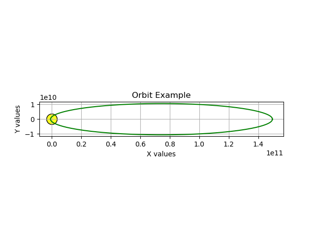
#!/usr/bin/env python
# -*- coding: utf-8 -*-

import math as m

import matplotlib.pyplot as plt

plt.axes().set_aspect('equal')
plt.xlabel("X values")
plt.ylabel("Y values")
plt.title("Orbit Example")
plt.grid()

# "Big G", universal gravitational constant
# https://physics.nist.gov/cgi-bin/cuu/Value?bg

G = 6.67430e-11

# Sun: https://nssdc.gsfc.nasa.gov/planetary/factsheet/sunfact.html

sunmass = 1.9885e30  # kilograms

# Earth: https://nssdc.gsfc.nasa.gov/planetary/factsheet/earthfact.html

earth_aphelion = 149.6e9  # greatest distance from the sun, meters
earth_velocity = 29.78e3  # initial velocity m/s

# model time slice seconds, default one hour

Δt = 3600.0

# x and y initial positions

yp = oy = 0
xp = earth_aphelion

# x and y initial velocities

yv = -earth_velocity
xv = 0

# arrays to contain orbital data

xvals = []
yvals = []

# precompute an acceleration term

accel_term = sunmass * -G * Δt

# model the orbit

while oy <= 0 or yp > 0:
  oy = yp

  # acquire gravitational acceleration
  acc = m.pow(xp**2+yp**2, -1.5) * accel_term

  # update velocity
  xv += xp * acc
  yv += yp * acc

  # update position
  xp += xv * Δt
  yp += yv * Δt

  # save values for later plotting
  xvals += [xp]
  yvals += [yp]

# draw the sun
plt.scatter(0, 0, marker='o', s=240, color='#ffff20', edgecolor='black')

# plot the orbit
plt.plot(xvals, yvals, color='g')

plt.savefig("gravity_example1.png")
As listed, the program produces this image:
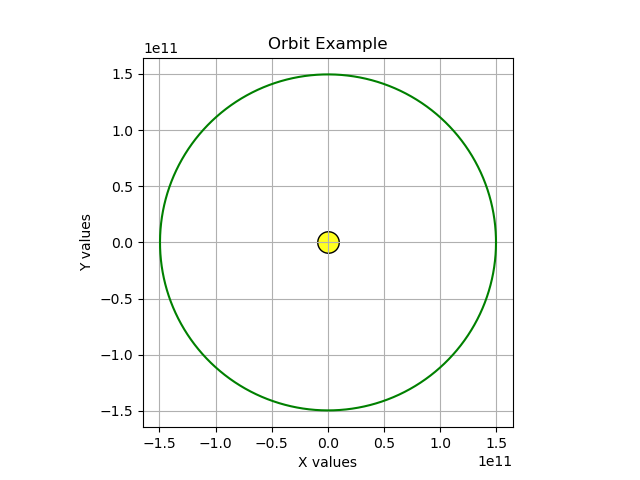
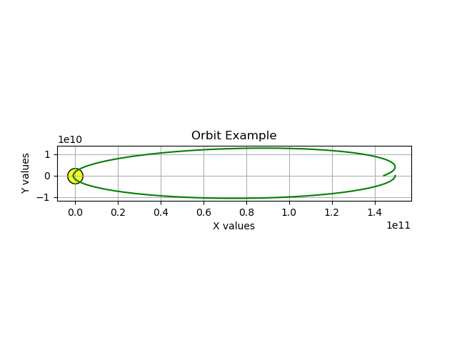
That's more or less Earth's orbit, without a few technical details like the absence of a small amount of elliptical eccentricity. Now let's make a change in the initial orbital velocity, see what happens. Change this line as shown:
yv = -earth_velocity * 0.5This change reduces the initial orbital velocity to 1/2 the original value. Here's the result:
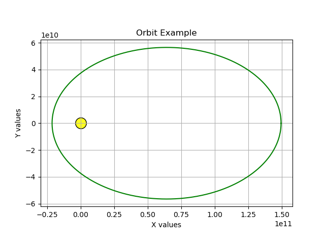
So by reducing the initial velocity, we create an oval or "eccentric" orbit with less energy than the original one. Now make this change:
yv = -earth_velocity * 0.25The new result:
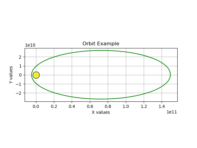
These are all realistic orbits with increasing amounts of eccentricity. Now for a radical change:
yv = -earth_velocity * 0.1Which creates this result:
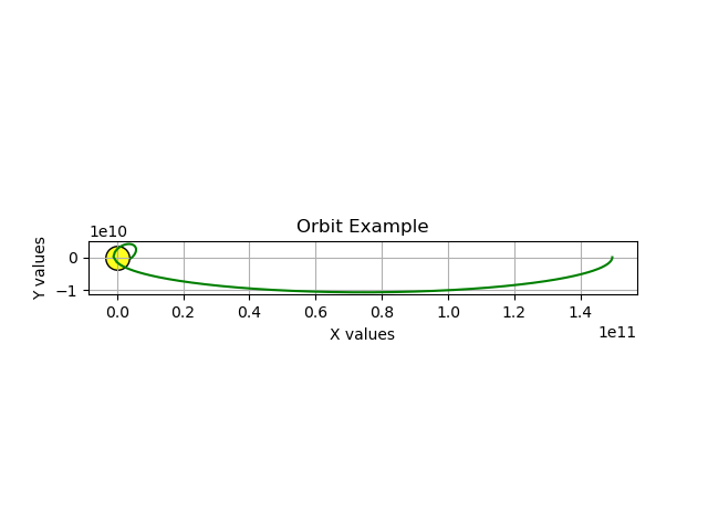
Wow — it looks as though our orbiting body crashed into the sun. But is this realistic? Remember that my sun drawing is much larger than the actual sun simply to be visible in these images, and the orbiting body ought to have orbited it as before, in a large but narrower oval. So it seems this outcome, this crash, isn't real physics. What went wrong?
It turns out that a computer orbital model is constrained by its parameters. For example if the selected time step Δt (say "delta-t") is large, the program will run fast — but in exchange, in the presence of rapid variations in velocity and acceleration, it may make errors.
In this program the default Δt value is 3600 seconds or one hour, meaning the model samples positions, velocities and accelerations at one-hour model-time intervals (not wall time). That time resolution appears to be inadequate to the task at hand. Let's try changing the Δt value, see what happens:
Δt = 600.0That's ten minutes in model time. Here's the result:
This is a better result, but there's some orbital precession visible at the right, that I doubt is part of physical reality. Let's try an even smaller Δt value:
Δt = 60.0One-minute time slices. The result:
That change appears to have fixed the model so it better reflects physical reality, but the program runs much more slowly. This is a classic computer numerical model tradeoff between physical accuracy and running time.
Takeaways:
- An accurate computer orbital model doesn't require many lines of code.
- A model written in Python or another fast-turnaround language allows quick program development but is often slow in execution.
- Other languages are better if both high accuracy and high speed are needed.
- The chosen model time step is a critical factor in model realism.
- A small time step may provide better accuracy and realism, but at the expense of running time.
Let's move away from orbital modeling to focus on another basic property of numerical differential equation solvers.
The basic idea of numerical differential equation solving is to write some code that executes an equation in small increments of time (or space etc.) and let the result evolve until some goal is achieved.
Here's a much simpler Python program (source) that also draws a kind of orbit, one that should calculate values for mathematical constants $𝜏$ and $𝜋$ as well as create a plot of the orbit. It's based on the idea that the circumference of a unit circle is equal to $𝜏$, roughly 6.283... or 2 times $𝜋$. The result is generated by a simple numerical differential equation:
#!/usr/bin/env python
# -*- coding: utf-8 -*-

import matplotlib.pyplot as plt

plt.axes().set_aspect('equal')
plt.xlabel("X values")
plt.ylabel("Y values")
plt.title("Differential Equation Example")
plt.grid()

# critical time step value
Δt = 0.25

ox = x = 0
y = 1
total = 0

xvals = []
yvals = []

while ox <= 0 or x > 0:
  ox = x
  x -= y * Δt
  y += x * Δt
  total += Δt
  xvals += [x]
  yvals += [y]

print(f"𝜏 = {total:.7f}")

print(f"𝜋 = {total/2:.7f}")

plt.plot(xvals,yvals)
plt.savefig("diffeq_example1.png")
This program generates a circle by exchanging small incremental numerical values between two variables — x and y — that represent horizontal and vertical space coordinates. The program detects that the circle is complete, prints its numerical results, generates a graph and exits.
For the first run I intentionally chose a Δt (say "delta-t") value that's too large. The program runs quickly and prints this:
𝜏 = 6.5000000
𝜋 = 3.2500000
And generates this graphic image:
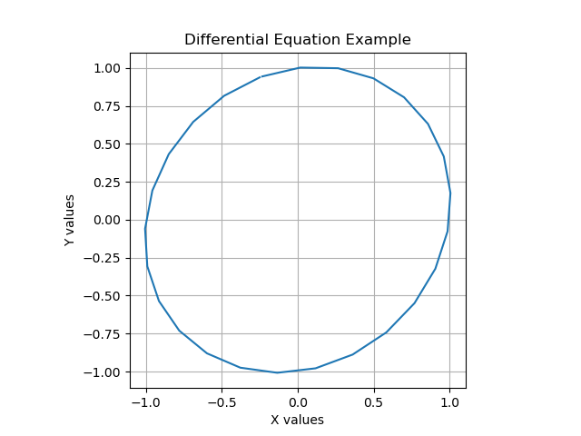
Clearly something is wrong — the circle is distorted and the resolution of the $𝜏$ and $𝜋$ values is poor.
So let's choose a better (smaller) Δt value:Δt = 1e-6;(1e-6 means one millionth or .000001)
And run the program again. The results:
𝜏 = 6.2831860
𝜋 = 3.1415930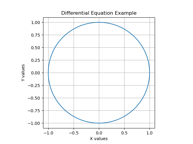
Essentially a perfect circle and a more accurate numerical outcome. It's a better result, but the Python program needed four seconds to produce it.
As a test, let's try a more extreme Δt value and see what happens:
Remember that 1e-7 is one tenth the size of 1e-6 (it's equal to 0.0000001). The result:Δt = 1e-7;𝜏 = 6.2831854 𝜋 = 3.1415927This is a better numerical result but required 38 seconds to execute on a fast modern computer (remember: it's Python). In fairness, much of the time was spent generating the graphic image, not computing the values.
Takeaways:
- Numerical solutions can be applied to many problems that (unlike this example) aren't accessible to pure mathematics.
- In some cases a numerical solution can require an absurd amount of computer power and time.
Here's an even simpler Python example (source) that, while computing a square root, reveals a hard limit to numerical modeling, one having to do with the finite resolution of computer numbers:
#!/usr/bin/env python
# -*- coding: utf-8 -*-

def showresult(x,Δx,n):
  print(f"x: {x:.15f}, Δx: {Δx:e}, pass: {n:2}")

y = 2.0
x = 1
n = 0

while True:

  Δx = (y - x * x) * 0.25

  if n % 2 == 0:
    showresult(x,Δx,n)

  n += 1

  ox = x
  x += Δx
  if ox == x: break

showresult(x,Δx,n)
As it runs, the program prints these intermediate results:
x: 1.000000000000000, Δx: 2.500000e-01, pass:  0
x: 1.359375000000000, Δx: 3.802490e-02, pass:  2
x: 1.409218280576169, Δx: 3.525959e-03, pass:  4
x: 1.413782668086311, Δx: 3.046419e-04, pass:  6
x: 1.414176579906956, Δx: 2.615021e-05, pass:  8
x: 1.414210389649588, Δx: 2.243452e-06, pass: 10
x: 1.414213290195495, Δx: 1.924586e-07, pass: 12
x: 1.414213539023941, Δx: 1.651034e-08, pass: 14
x: 1.414213560370054, Δx: 1.416364e-09, pass: 16
x: 1.414213562201261, Δx: 1.215048e-10, pass: 18
x: 1.414213562358354, Δx: 1.042344e-11, pass: 20
x: 1.414213562371831, Δx: 8.941181e-13, pass: 22
x: 1.414213562372987, Δx: 7.671641e-14, pass: 24
x: 1.414213562373086, Δx: 6.550316e-15, pass: 26
x: 1.414213562373094, Δx: 5.551115e-16, pass: 28
x: 1.414213562373095, Δx: 1.110223e-16, pass: 30
At pass 30 the program detects a terminating condition and exits.
That's a pretty good square root result (as before, there are more efficient ways to calculate square roots). But notice the final Δx value, 1.110223e-16. The program exits when there are no more detected changes to the desired x result. But just before the equality test:
if ox == x: break... we added Δx to x:
x += ΔxShouldn't that have changed the x value?
As it happens, when you add or subtract two computer numbers, the numeric processor must first shift one of the numbers (align the mantissas) until the two exponents are equal — this is a requirement for adding and subtracting numbers. But typical "double-precision" computer numbers have 52 binary bits of resolution, which provide only about 15 base-10 digits. A brief digression:
For two number bases $A$ and $B$: \begin{equation} nd_B = \frac{nd_A \log(A)}{\log(B)} \end{equation} Where:
- $A,B$ = number bases, example 2 and 10.
- $nd_A,nd_B$ = number of available digits in $A$ and $B$.
So, for an IEEE 754 double-precision variable with a 52-binary-bit mantissa:
\begin{equation} \frac{52 \log(2)}{\log(10)} = 15.65\, \text{base-10 digits} \end{equation}This means that, even though the earlier value of 5.551115e-16 (in pass 28) was just large enough to change x, the final Δx value of 1.110223e-16 (pass 30) was too small and the algorithm terminated. Here's a Python REPL example that shows why:
>>> 1 + 5e-16 == 1
False
>>> 1 + 2e-16 == 1
False
>>> 1 + 1e-16 == 1
True
I include this example to show that, due to finite numerical precision, hard limits exist in computer numerical modeling. There are other limits, but if two numbers differ enough in magnitude and the algorithm relies on addition/subtraction, you may no longer be able to change one variable with the other and your algorithm will fail.
I also include this example because of its relevance to an optimization problem I encountered during my Lagrange orbit study, in which I performed a binary search for orbital parameters that could keep the JWST in a stable Lagrange orbit for up to two years with no fuel expenditure, but only if the initial orbital velocity was set to an excruciatingly precise value calculated to ten decimal places — details in this article's Section 3.
Takeaways:
- In numerical differential equation solvers, there are many important parameters, but the step size is at the top of the list — it can't be too large or too small.
- If the step size is too large the outcome may be too coarsely generated to be useful.
- If the step size is too small it may not be able to influence the model's variables and the code may run forever, waiting for a condition that may never arise.
- This means a critical design goal should be to establish a "Goldilocks zone" of acceptable step sizes, outside of which the algorithm loses its way.
The is an optional section for those who want to understand the mathematical details of the gravity simulation. It can be safely skipped by those with little interest in mathematics.
We start with the already-presented Newtonian gravitational equation:
\begin{equation} \displaystyle f = G \frac{m_1 m_2}{r^2} \end{equation}Where:
- $f$ = Force, units Newtons.
- $G$ = Universal gravitational constant.
- $m_1,m_2$ = the masses of two bodies influenced by gravity, units kilograms.
- $r$ = Distance between $m_1$ and $m_2$, meters.
In the examples above we've only applied gravitational force to single objects, each with respect to a stationary attracting body located at the three-dimensional coordinate origin {0,0,0}, which greatly simplifies the mathematics. But in a full gravitational model with multiple moving bodies, for each slice of time we must apply the Newtonian equation to each pair of masses, regardless of their locations and separations.
This means each body must experience a vector sum of its attraction to all other bodies in the simulation. For example our moon is attracted to Earth, but also to the Sun, to Jupiter, and so forth. This means the computation workload increases roughly as the square of the number of interacting bodies as shown in this table:
(+ = computation required)
Sun Mercury Venus Earth Moon JWST Mars Jupiter Uranus Neptune Sun + + + + + + + + + Mercury + + + + + + + + + Venus + + + + + + + + + Earth + + + + + + + + + Moon + + + + + + + + + JWST + + + + + + + + + Mars + + + + + + + + + Jupiter + + + + + + + + + Uranus + + + + + + + + + Neptune + + + + + + + + + The above table shows the simulation members in my James Webb Space Telescope orbital study. I would have excluded Earth's relatively low-mass moon to save computation time but as it turns out, because of its proximity to the JWST, our moon has a dramatic effect on the spacecraft's Lagrange point L2 orbit, both with regard to location and stability.
For a given simulation and as the above table shows, the sum $S$ of gravitational force vector computations is:
\begin{equation} \displaystyle S = N^2-N \end{equation}for $N$ interacting bodies, which for this example equals 90 computations per simulator time slice.
This is why supercomputers are required to study star clusters and galaxies, where the number of interacting bodies easily exceeds any practical limit. In fairness, in such studies, particular bodies are eliminated from the computation based on their small mass and/or large distance.
Details
Here are the steps in this study's orbital force computation:
For each pair of bodies $\vec{a},\vec{b}$ in the above table, a position differential vector $(\vec{a}-\vec{b})$ is created:
\begin{equation} \displaystyle \{dx, dy, dz\} = \vec{a}\{x,y,z\} - \vec{b}\{x,y,z\} \end{equation}A scalar $r$ is created that represents the radial distance between the bodies $(a,b)$:
\begin{equation} \displaystyle r = \sqrt{dx^2+dy^2+dz^2} \end{equation}With the $r$ value from equation (7), a gravitational force scalar $f$ is computed:
\begin{equation} \displaystyle f = - \frac{G m_1 m_2}{r^2} \end{equation}Using the $r$ value from equation (7), a normalizing scalar $\hat{r}$ is created to constrain the computed result to the range -1 <= $\{dx, dy, dz\}$ <= 1:
\begin{equation} \displaystyle \hat{r} = \frac{1}{r} = \frac{1}{\sqrt{dx^2+dy^2+dz^2}} \end{equation}Using this computation strategy, for each pair of bodies and for each simulation step $n$:
A body's velocity vector is updated by the position differential vector $\{dx, dy, dz\}$ (equation 6) multiplied by the gravitational acceleration scalar $f$ (equation 8), the normalizing scalar $\hat{r}$ (equation 9) and the simulation time slice $\Delta t$:
\begin{equation} \displaystyle \vec{v}_{n+1} = \vec{v}_{n} + \{dx, dy, dz\} \, \hat{r} \, f \, \Delta t \end{equation}The body's position vector is then updated by the computed velocity times $\Delta t$:
\begin{equation} \displaystyle \vec{p}_{n+1} = \vec{p}_{n} + \vec{v}_{n+1} \, \Delta t \end{equation}It turns out that in this strategy, optimizations are possible — the computation workload can be reduced using algebraic manipulation. Because the normalizing scalar $\hat{r}$ is multiplied by the force scalar $f$ to produce an acceleration vector $\vec{a}$, we can proceed like this:
Normalizing scalar $\hat{r}$ (equation 9) can be expressed like this:
\begin{equation} \displaystyle \hat{r} = \frac{1}{r} = \frac{1}{\sqrt{dx^2+dy^2+dz^2}} \rightarrow (dx^2+dy^2+dz^2)^{-1/2} \end{equation}Radial distance scalar $r$ (equation 7) can be expressed like this:
\begin{equation} \displaystyle r = \sqrt{dx^2+dy^2+dz^2} \rightarrow (dx^2+dy^2+dz^2)^{1/2} \end{equation}Force scalar $f$ (equation 8) can be expressed like this:
\begin{equation} \displaystyle f = - \frac{G m_1 m_2}{r^2} \rightarrow -G m_1 m_2 \, (dx^2+dy^2+dz^2)^{-1} \end{equation}Using expressions from equations (12) and (14) , the acceleration vector $\vec{a}$ now looks like this:
\begin{equation} \displaystyle \vec{a} = \{dx, dy, dz\} -G m_1 m_2 \, (dx^2+dy^2+dz^2)^{-1} \, (dx^2+dy^2+dz^2)^{-1/2} \end{equation}Through algebraic simplification, acceleration $\vec{a}$ becomes:
\begin{equation} \displaystyle \vec{a} = \{dx, dy, dz\} -G m_1 m_2 \, (dx^2+dy^2+dz^2)^{-3/2} \end{equation}The result of this optimization is an acceleration vector that represents an absolute minimum of computation overhead and that accurately represents orbital gravitation in three dimensions.
Takeaways:
- While computing orbits, when possible avoid trigonometric and other exotic, time-absorbing functions.
- For speed of execution, pare the math down to its most basic elements without sacrificing accuracy.
- Remember the critical role played by Δt ("delta-t"), the simulation's time step, which determines the outcome's accuracy and realism. This value has a distinctive "Goldilocks" property -- not too big, not too small.
In the next section of this article I discuss programming issues and the best computer languages to process this physical model.
| Home | | Orbital Modeling | | | | Share This Page |