

 Share This Page
| Home | | Orbital Modeling | | | | Share This Page |
Section 2. Programming/Language Issues
— P. Lutus — Message Page —
Copyright © 2022, P. Lutus
Most recent update:
In this section I discuss computer programming and language issues, and maybe advocate in favor of Rust a bit. Section 1 of this article covered the theory and mathematics behind orbital modeling, this section deals with practical issues leading to usable results.
Over time computers are becoming faster and have more memory to deal with resource-intensive solutions, but in spite of this, efficient programs should always be given a high priority.
Obviously the meaning of "efficient program" changes over time, since the time required to create and test a program must be considered alongside the program's execution speed.
In this section I test my orbital model in several computer languages, describe their advantages and drawbacks, and show a speed comparison between them when running an identical orbital simulation. In these tests each language is required to demonstrate the orbital algorithm's innate precision while logging its execution speed.
I wrote each of the test programs to be as close to identical as practical. Each sets up a year-long simulated Earth orbit using published constants like "Big G", orbital parameters for the Sun (primarily mass) and Earth (detailed orbital properties):
• "Big G", the universal gravitational constant: NIST: Fundamental Physical Constants • Solar data: Sun Fact Sheet (NASA) • Earth data: Earth Fact Sheet (NASA) Earth's orbit has a small amount of eccentricity (e = 0.0167), consequently it has a point of greatest distance from the sun (aphelion) and least (perihelion). In keeping with the principle of orbital energy conservation these points are accompanied by different velocities. For my model to be regarded as valid, a simulated orbit had to duplicate all these parameters (distances, velocities, energy) in complete agreement with published values.
In each test case, the execution time in milliseconds was established by bracketing the execution loop with two time recordings, as close to the execution loop as possible, so no compilation or I/O tasks were included in the recorded times.
As they run, the test programs print the orbital setup data, then, on completion of the simulation run, they print detailed results for comparison with published values. For each program the output looks like this:
Model: Earth orbit
Simulator step size Δt: 10.00 seconds
Calculated/measured orbital parameters:
  Orbital radius meters:
    max (aphelion):   1.521000e11
    min (perihelion): 1.470950e11
  Orbital velocity m/s:
    max: 3.028790e4
    min: 2.929125e4
  Orbital energy joules (should be constant):
    mean: -2.649179e33
Simulation results:
  Iterations: 3155760
  Orbital radius meters:
    max: 1.521000e11
    min: 1.470950e11
  Orbital velocity m/s:
    max: 3.028790e4
    min: 2.929125e4
  Orbital energy joules:
    max:   -2.649179e33
    min:   -2.649179e33
    error: 0.0000067%

Elapsed algorithm time: 114.632 ms
The runtime at the bottom of the list is from the Rust version of my program. To be regarded as valid and with the exception of runtime, each of the programs had to show the exact results as shown above, in particular the error value, which in the test series was the same for each program.
A small digression. The error value is acceptable, quite small, but it can be made smaller by reducing the Δt value, which nearly always represents a tradeoff between precision and execution time. But remember — a change in the Δt value that gains an order of magnitude in orbital precision, will generally also gain an order of magnitude in execution time.
Because an elliptical orbit should have constant energy, I've always regarded the smallest practical energy deviation as a litmus test for the quality of an orbital simulation.
I wrote a Python script that automatically compiled (when needed) and ran each of the language test cases and acquired the timing results. This chart was created automatically using just-collected test results:
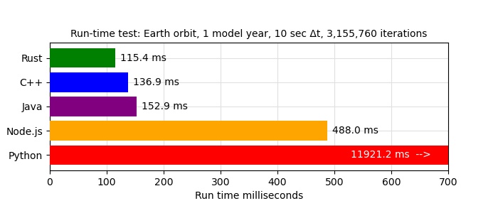
First: yes, boys and girls, this chart isn't lying — in a number-crunching task Rust is 103 times faster than Python (C++ is 87 times faster).
Second, because the above Rust/C++ comparison may be regarded as controversial, here are the compilation command-lines I used for Rust and C++:
- Rust: "$ cargo run --release main.rs"
- C++: "$ g++ -O2 *.cpp && ./a.out"
I tried several C++ compilation options to improve execution speed and settled on the above based on the outcome, which seemingly couldn't be improved upon.
Source archives for each of the test languages are included below (GPL 3.0 open source) so readers can run their own tests and see if any mistakes have been made. The archives are compatible with, and are meant to be used with, the open-source VS Code development environment:
• Rust: Rust.zip • C++: C++.zip • Java: Java.zip • Node.js: Node.js.zip • Python: Python.zip
Once I realized Rust outperformed all the other languages I tested, I moved my primary coding activity there and tried to come up to speed in what was for me a new language. Rust's advantages were immediately apparent — no garbage collector, no memory leaks, no need to formally create and destroy class instances and explicitly manage memory as one does in C++ and elsewhere. No header files that must be kept synchronized with source files. And an excellent Rust development environment in VS Code that immediately alerts you to errors without waiting for the compiler to complain.
I chose Rust for this project based on its clean programming model and its speed. Its improved security against attack isn't an issue for this project, but for general programming that's certainly a reason to consider learning Rust. I think young programmers should at least acquire some familiarity with Rust, as a hedge against a future where Rust itself or similarly designed languages are likely to become the norm.
I have to tell you, this isn't my first gravity simulator. My very first was a kind of computer game, before personal computers even existed. In 1976 I wrote the game on a programmable calculator (HP-25), then I published it in a science magazine and people played the game using graph paper as a display — full description here.
My next gravity model covered all solar system planets (including Pluto in those days), written on another programmable calculator (HP-67). After publication, some people at JPL and elsewhere used it during the Mars Viking lander mission — full description here.
The reason for my program's popularity was that people at JPL who needed reasonably accurate planetary positions had two choices:
- Punch some 80-column data/code cards, submit the cards to the computer center, then wait 24 hours for a result.
- Grab their HP calculators and use my program to get less accurate but useful results right away.
Remember — this was 1977, personal computers hadn't arrived yet, people in my line of work owned at least one slide rule, and in my NASA subcontractor office I put a glass box on the wall that said "In Emergency Break Glass". Inside the box was an abacus.
My early models relied too much on trigonometry and similarly clunky solutions, primarily because I had no way to test better algorithms in a time-efficient way. Entering instructions into a programmable calculator isn't remotely like modern programming -- for example one couldn't insert a new instruction between two existing ones. In fact, to insert missing instructions into an HP-25 program, you had to do this (quoting directly from the online HP-25 instruction manual):
Adding Instructions If you have recorded a medium-sized program and have left out a crucial sequence of keystrokes right in the middle, you do not have to start over. The missing sequence of keystrokes can be recorded in the available steps following your program. You can then use the GTO key to make an unconditional branch to the sequence when it is needed and then make a second unconditional branch back to the main part of your program at the end of the sequence. [ emphasis added ]I wish I was making this up. Oh, did I mention there was no non-volatile storage (on the HP-25)? If you turned the calculator off or the battery died, you had to start over.
One irony of my newer numerical models is that computers are now so fast that I can test different algorithms quickly, weed out inefficient methods and cull redundant operations, all on a computer where the resulting execution-time improvements make much less difference than they would have in the 1970s.
In the next section of this article I show the results of my JWST Lagrange orbit model, which is by far the most ambitious of my solar system models.
| Home | | Orbital Modeling | | | | Share This Page |